An introduction to variational autoencoders
November 04, 2023
We are all latent variable models
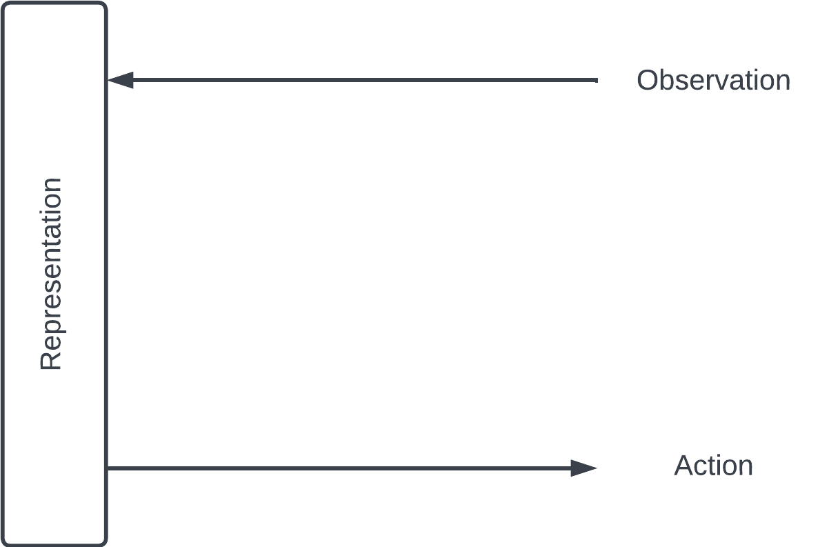
Here's one way of looking at learning. We interact with the world through observing (hearing, seeing) and acting (speaking, doing). We encode our observations about the world into some representation in our brain – and refine it as we observe more. Our actions reflect this representation.
Encoding & decoding
Imitation is an effective way to learn that engages both observation and action. For example, babies repeat the words of their parents. As they make mistakes and get corrected, they hone their internal representation of the words they hear (the encoder) as well as the way they create their own words from that representation (the decoder).
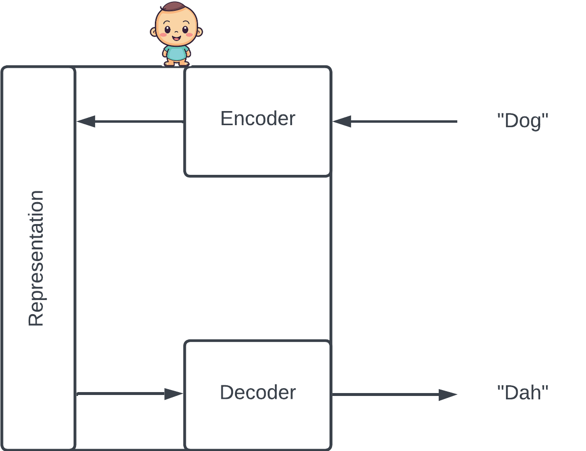
The baby tries to reconstruct the input via its internal representation. In this case, he incorrectly reconstructs "Dog" as "Dah".
Crudely casting this in machine learning terms, the representation is a vector called a latent variable, which lives in the latent space. The baby is a latent variable model engaged in a task called reconstruction.
A note on notation: when talking about probability, I find it helpful to make explicit whether something is fixed or a variable in a distribution by making fixed things bold. For example, is a fixed vector, is a conditional distribution over possible values of . is a number between and (a probability) while is a distribution, i.e. a function of .
Given observation , the encoder is a distribution over the latent space; knowing , the encoder tells us which latent variables are probable. To obtain some , we sample from .
Similarly, given some latent variable , the decoder is a distribution . When sampled from, the decoder produces a reconstructed .
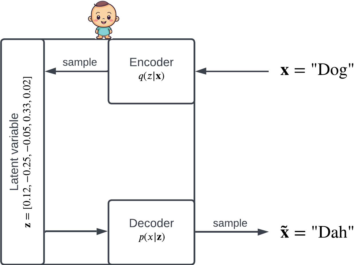
The latent variable is a vector . The encoder and decoder are both conditional distributions.
The variational autoencoder
When neural networks are used as both the encoder and the decoder, the latent variable model is called a variational autoencoder (VAE).
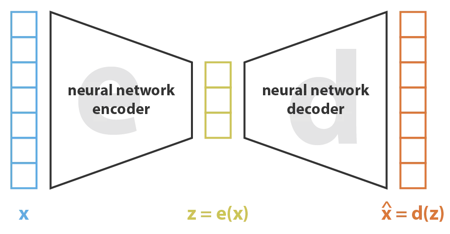
Variational autoencoders are a type of encoder-decoder model. Figure from this blog post.
The latent space has fewer dimensions than the inputs, so encoding can be viewed as a form of data compression. The baby doesn't retain all the details of each syllable heard – the intricate patterns of each sound wave – only their compressed, salient features.
Evaluation reconstruction
A good model at reconstruction often gets it exactly right: . Given some input , let's pick some random and look at : the probability of reconstructing the input perfectly. We want this number to be big.
But that's not really fair: what if we picked a that the encoder would never choose? After all, the decoder only sees the latent variables produced by the encoder. Ideally, we want to assign more weight to 's that the encoder is more likely to produce:
The weighted average is also known as an expectation over , written as :
If is high, we can tell our model that it did a good job.
Regularization
Neural networks tend to overfit. Imagine if our encoder learns to give each input it sees during training its unique corner in the latent space, and the decoder cooperates on this obvious signal.
We would get perfect reconstruction! But we don't want this. The model failed to capture the close relationship between "Dog" and "Doggy". A good, generalizable model should treat them similarly by assigning them similar latent variables. In other words, we don't want our model to merely memorize and regurgitate the inputs.
While a baby's brain is exceptionally good at dealing with this problem, neural networks need a helping hand. One approach is to guide the distribution of the latent variable to be something simple and nice, like the standard normal:
We talked previously about KL divergence, a similarity measure between probability distributions; tells us how far the encoder has strayed from the standard normal.
The loss function
Putting everything together, let's write down the intuition that we want the model to 1) reconstruct well and 2) have an encoder distribution close to the standard normal:
This is the Evidence Lower BOund (ELBO) – we'll explain the name later! – a quantity we want to maximize. The expectation captures our strive for perfect reconstruction, while the KL divergence term acts as a penalty for complex, nonstandard encoder distributions. This technique to prevent overfitting is called regularization.
In machine learning, we're used to minimizing things, so let's define a loss function whose minimization is equivalent to maximizing ELBO:
Some notes
Forcing to be standard normal might seem strange. Don't we want the distribution of to be something informative learned by the model? I think about it like this: the encoder and decoder are complex functions with many parameters (they're neural networks!) and they have all the power. Under a sufficiently complex function, can be transformed into anything you want. The art is in this transformation.
On the left are samples from a standard normal distribution. On the right are those samples mapped through the function . VAEs work in a similar way: they learn functions like that create arbitrary complex distributions. Figure from 1.
So far, we talked about variational autoencoders purely through the lens of machine learning. Some of the formulations might feel unnatural, e.g. why do we regularize in this weird way?
Variational autoencoders are actually deeply rooted in a field of statistics called variational inference – the first principles behind these decisions. That is the subject of the next section.
Variational Inference
Here's another way to look at the reconstruction problem. The baby has some internal distribution over the latent space: his mental model of the world. Every time he hears and repeats a word, he makes some update to this distribution. Learning is nothing but a series of these updates.
Given some word , the baby performs the update:
is the prior distribution (before the update) and is the posterior distribution (after the update). With each observation, the baby computes the posterior and uses it as the prior for the next observation. This approach is called Bayesian inference because to compute the posterior, we use Bayes rule:
This formula seems obvious from the manipulation of math-symbols , but I've always found it hard to understand what it actually means. In the rest of this section, I will try to provide an intuitive explanation.
The evidence
One quick aside before we dive in. , called the evidence, is a weighted average of probabilities conditional on all possible latent variables :
is an averaged opinion across all 's that represents our best guess at how probable is.
When the latent space is massive, as in our case, is infeasible to compute.
Bayesian updates
Let's look at Bayes rule purely through the lens of the distribution update: .
- I have some preconception (prior),
- I see some (e.g. "Dog")
- Now I have some updated mental model (posterior),
How should the new observation influence my mental model? At the very least, we should increase , the probability we assign to observing , since we literally just observed it!
Under the hood, we have a long vector with a probability value for each possible in the latent space. With each observation, we update every value in .
Click the update button to adjust based on some observed . At each step, the probability associated with each is updated. The probabilities are made up.
We can think of these bars (probabilities) as knobs we can tweak to adjust our mental model to better fit each new observation (without losing sight of previous ones).
Understanding the fraction
Let's take some random . Suppose leads me to think that is likely, say 60% (), while the averaged opinion is only 20% (). Given that we just observed , did better than average. Let's promote it by bumping its assigned probability by:
The posterior is:
Conversely, if leads me to think that is unlikely, say 20% (), while the averaged opinion is 60% (), then did worse than the average. Let's decrease its assigned probability:
Either by promoting an advocate of or demoting a naysayer, we 1) adjust the latent distribution to better fit and 2) bring up the average opinion, .
That's the essence of the update rule: it's all controlled by the fraction .
Approximating the posterior
As we mentioned, the evidence is impossible to compute because it is a sum over all possible latent variables. Since is the denominator of the Bayesian update, this means that we can't actually compute the posterior distribution – we need to approximate it.
The two most popular methods for approximating complex distributions are Markov Chain Monte Carlo (MCMC) and variational inference. We talked about MCMC previously in various contexts. It uses a trial-and-error approach to generate samples from which we can then learn about the underlying complex distribution.
In contrast, variational inference looks at a family of distributions and tries to pick the best one. For illustration, we assume the observations follow a normal distribution and consider all distributions we get by varying the the mean and variance.
Try adjusting the the mean and variance of the normal distribution to fit the observations (blue dots). In essense, varational inference is all about doing these adjustments.
Variational inference is a principled way to vary these parameters of the distribution (hence the name!) and find a setting of them that best explains the observations. Of course, in practice the distributions are much more complex.
In our case, let's try to use some distribution to approximate . We want to be as similar to as possible, which we can enforce by minimizing the KL divergence between them:
If the KL divergence is , then perfectly approximates the posterior .
The Evidence Lower Bound (ELBO)
If you're not interested in the mathematical details, this section can be skipped entirely. TLDR: expanding out yields the foundational equation of variational inference at the end of the section.
By definition of KL divergence and applying log rules:
Apply Bayes rule and log rules:
Move out of the expectation because it doesn't depend on :
Separate terms into 2 expectations and group with log rules:
The first expectation is a KL divergence: . Rewriting and rearranging:
This is the central equation in variational inference. The right hand side is exactly what we have called the evidence lower bound (ELBO).
Interpreting ELBO
From expanding , we got:
Since cannot be negative , is a lower bound on the (log-)evidence, . That's why it's called the evidence lower bound!
Adjust the slider to mimic the process of maximizing ELBO, a lower bound on the (log-)evidence. Since is the "distance" between ELBO and , our orginial goal of minimizing it brings ELBO closer to .
Let's think about the left hand side of the equation. Maximizing ELBO has two desired effects:
-
increase . This is our basic requirement: since we just observed , should go up!
-
minimize , which satisfies our goal of approximating the posterior.
VAEs are neural networks that do variational inference
The machine learning motivations for VAEs we started with (encoder-decoder, reconstruction loss, regularization) are grounded in the statistics of variational inference (Bayesian updates, evidence maximization, posterior approximation). Let's explore the connections:
Variational Inference | VAEs (machine learning) | |
|---|---|---|
We couldn't directly compute the posterior in the Bayesian update, so we try to approximate it with . | is the encoder. Using a neural network as the encoder gives us the flexibility to do this approximation well. | |
fell out as a term in ELBO whose maximization accomplishes the dual goal of maximizing the intractable evidence, , and bringing close to . | is the decoder, also a neural network. is the probability of perfect reconstruction. It makes sense to strive for perfect reconstruction and maximize this probability. | |
is the prior we use before seeing any observations. is a reasonable choice. It's a starting point. It would take a lot of observations that disobey to, via Bayesian updates, convince us of a drastically different latent distribution. | Our encoder and decoder are both neural networks. They're just black-box learners of complex distributions with no concept of priors. They can easily conjure up a wildly complex distribution – nothing like – that merely memorizes the observations, a problem called overfitting. To prevent this, we constantly nudge the encoder towards , as a reminder of where it would have started if we were using traditional Bayesian updates. When viewed this way, is a regularization term. |
Modeling protein sequences
Pair-wise models are limiting
In a previous post, we talked about ways to extract the information hidden in Multiple Sequence Alignments (MSAs): the co-evolutionary data of proteins. For example, amino acid positions that co-vary in the MSA tend to interact with each other in the folded structure, often via direct 3D contact.
MSA
An MSA contains different variants of a sequence. The structure sketches how the amino acid chain might fold in space (try dragging the nodes). Hover over each row in the MSA to see the corresponding amino acid in the folded structure. Hover over the blue link to highlight the contacting positions.
We talked about position-wise models that look at each position and pair-wise models that consider all possible pairs of positions. But what about the interactions between 3 positions? Or even more? Those higher-order interactions are commonplace in natural proteins but modelling them is unfortunately computationally unfeasible.
Variational autoencoders for proteins
Let's imagine there being some latent variable vector that explains all interactions – including higher-order ones.
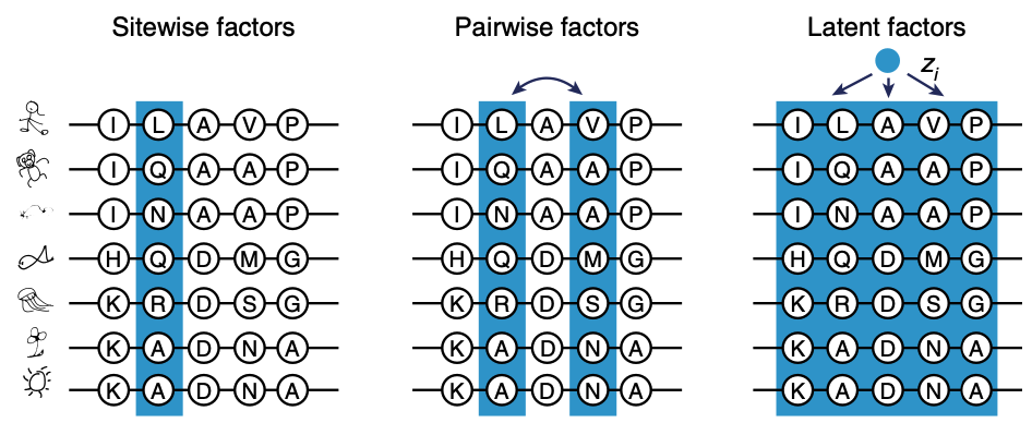
Applying latent variable models like VAEs to MSAs. Figure from 2.
Like the mysterious representation hidden in the baby's brain, we don't need to understand exactly how it encodes these higher-order interactions; we let the neural networks, guided by the reconstruction task, figure it out.
In this work, researchers from the Marks lab did exactly this to create a VAE model called DeepSequence. I will do a deep dive on this model – and variants of it – in the next post!
Further reading
I am inspired by this blog post by Jaan Altosaar and this blog post by Lilian Weng, both of which are superb and go into more technical details.
Also, check out the cool paper from the Marks lab applying VAEs to protein sequences. You should have the theorical tools to understand it well.
References
Doersch, C. Tutorial on Variational Autoencoders. arXiv (2016).
Riesselman, A.J. et al. Deep generative models of genetic variation capture the effects of mutations. Nat Methods 15, 816–822 (2018).
Doersch, C. Tutorial on Variational Autoencoders. arXiv (2016).
Riesselman, A.J. et al. Deep generative models of genetic variation capture the effects of mutations. Nat Methods 15, 816–822 (2018).
- We also use log probability for mathematical convenience.
- , from the definition of conditional probability. To see Bayes rule, simply take and divide both sides by .
- This is a property of KL divergence.